The McFarthest Point

Ever wanted to just get away as far as possible ...from any McDonald's? You're in luck, I calculated the exact coordinates inside the United States where you can feel free again!

The McFruthest Point is the point in the US that is as far away as possible from any McDonald's locations.

Keep reading to see how math and some GIS magic helped me in this monumental scientific achievement.

Data

First of all, we need some McCoordinates. I haven't found any dataset from the current year sadly, but this one from Kaggle contains almost 14000 locations, which should be great to start with. If anybody has a newer McCoordinate dataset, please let me know – would love to update my findings.

The second dataset we'll use is a cartographic boundary file of every state in the US, straight from the Census bureau. We will need this to constrain our calculations to US soil.

We'll use Geopandas to read our source data and to calculate anything geolocation related.

df["coords"] = df["geometry.coordinates"].apply(lambda x: eval(x))
df["latitudes"] = df["coords"].apply(lambda x: x[1])
df["longitudes"] = df["coords"].apply(lambda x: x[0])
gdf = gpd.GeoDataFrame(df, geometry=gpd.points_from_xy(df.longitudes, df.latitudes))

# filter latitudes higher than 50 (Alaska and Hawaii)
gdf = gdf[gdf.latitudes < 50]

states = gpd.read_file("tl_2022_us_state.shp")
states = states.to_crs("EPSG:4326")
non_continental = ['HI', 'VI', 'MP', 'GU', 'AK', 'AS', 'PR']
us49 = states
for n in non_continental:
    us49 = us49[us49.STUSPS != n]

After loading both datasets and consolidating them into the same coordinate system, we can quickly plot out all the locations in our dataset.

gdf.crs = "EPSG:4326"
gdf_proj = gdf.to_crs(us49.crs)

fig, ax = plt.subplots(figsize=(20, 20))

us49.plot(ax=ax, color="grey")
gdf_proj.plot(ax=ax, color="white", markersize=2)

ax.axis("off")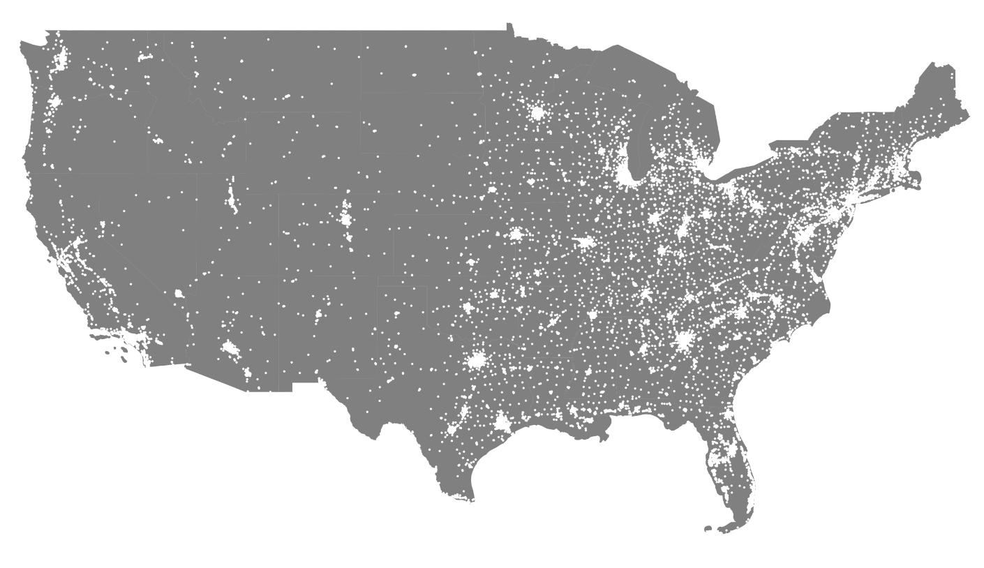

In this map, every white point is a restaurant. There's a lot, huh? And this is years-old data! Anyway, let's continue.

Data ... science?

So the next step is to find the point on this map that is the furthest away possible from any of these white little dots.

The solution to this problem lies in the Voronoi diagram. This diagram is a way to divide a plane into regions based on a set of points, where each region contains the point that is closest to it. The boundaries of these regions are straight lines that intersect at points called vertices.

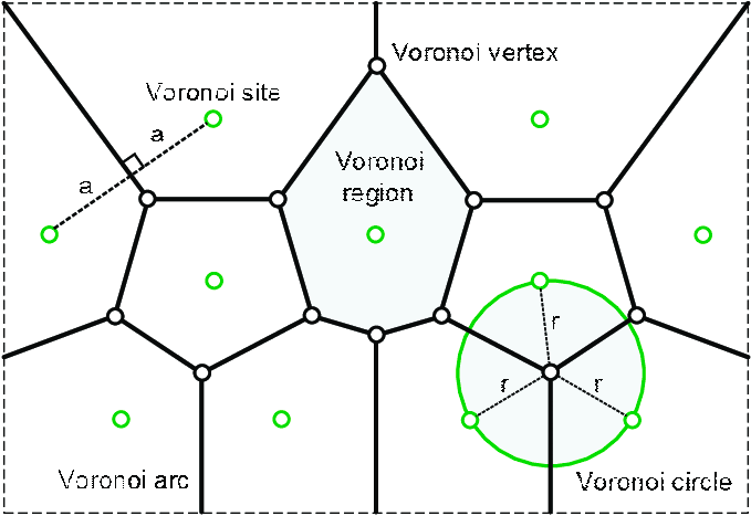
These vertices have a special property: they are equidistant to at least three points from the original set. By finding the sparsest point on the plane, which is either a vertex in the Voronoi diagram, the intersection of an edge in the Voronoi diagram with the boundary of the plane, or one of the corners of the plane, we can determine the farthest location from any McDonald's.

Calculating the Voronoi diagram can be done using standard algorithms in O(n log n) time, where n is the number of points in the original set. Once we have the diagram, we can find the sparsest point in linear time by knowing which Voronoi regions each vertex/edge is adjacent to and measuring the distance to the corresponding point in the original set.

Alright, so how does this look in Python? And does it actually work? Let's see!

Implementation

First, we prepare the shape background we use to constrain our Voronois vertices onto the continental US, otherwise, they would just fly away into infinity.

I'll be using Shapely and the geovoronoi library for most of the following computations.

from geovoronoi import points_to_coords
from shapely.ops import unary_union

area_shape = unary_union(us49.geometry)
coords = points_to_coords(gdf_proj.geometry)

Great, after that's done, we can calculate the actual diagram values.

from shapely import MultiPoint, Point
from shapely.ops import voronoi_diagram

points = MultiPoint([Point(x, y) for x, y in coords])
regions = voronoi_diagram(points)

Simple, right?! Well, we're not done yet! This diagram spans to infinity, which means that the furthest possible point would be somewhere infinitely far away as well. So we need to restrict our diagrams to a closed 2d plane. After we get rid of the pesky infinite vertices, we'll map the diagram onto our shape background.

This shape background are will be the convex hull defined by the polygons of the 49 continental US states. Let's see how this works.

To reconstruct our Voronoi diagram in a finite 2d plane, I'll be using this function:

import numpy as np
import matplotlib.pyplot as plt
from scipy.spatial import Voronoi

def voronoi_finite_polygons_2d(vor, radius=None):
    """
    Reconstruct infinite voronoi regions in a 2D diagram to finite
    regions.

    Parameters
    ----------
    vor : Voronoi
        Input diagram
    radius : float, optional
        Distance to 'points at infinity'.

    Returns
    -------
    regions : list of tuples
        Indices of vertices in each revised Voronoi regions.
    vertices : list of tuples
        Coordinates for revised Voronoi vertices. Same as coordinates
        of input vertices, with 'points at infinity' appended to the
        end.

    """

    if vor.points.shape[1] != 2:
        raise ValueError("Requires 2D input")

    new_regions = []
    new_vertices = vor.vertices.tolist()

    center = vor.points.mean(axis=0)
    if radius is None:
        radius = vor.points.ptp().max()

    # Construct a map containing all ridges for a given point
    all_ridges = {}
    for (p1, p2), (v1, v2) in zip(vor.ridge_points, vor.ridge_vertices):
        all_ridges.setdefault(p1, []).append((p2, v1, v2))
        all_ridges.setdefault(p2, []).append((p1, v1, v2))

    # Reconstruct infinite regions
    for p1, region in enumerate(vor.point_region):
        vertices = vor.regions[region]

        if all(v >= 0 for v in vertices):
            # finite region
            new_regions.append(vertices)
            continue

        # reconstruct a non-finite region
        ridges = all_ridges[p1]
        new_region = [v for v in vertices if v >= 0]

        for p2, v1, v2 in ridges:
            if v2 < 0:
                v1, v2 = v2, v1
            if v1 >= 0:
                # finite ridge: already in the region
                continue

            # Compute the missing endpoint of an infinite ridge

            t = vor.points[p2] - vor.points[p1] # tangent
            t /= np.linalg.norm(t)
            n = np.array([-t[1], t[0]])  # normal

            midpoint = vor.points[[p1, p2]].mean(axis=0)
            direction = np.sign(np.dot(midpoint - center, n)) * n
            far_point = vor.vertices[v2] + direction * radius

            new_region.append(len(new_vertices))
            new_vertices.append(far_point.tolist())

        # sort region counterclockwise
        vs = np.asarray([new_vertices[v] for v in new_region])
        c = vs.mean(axis=0)
        angles = np.arctan2(vs[:,1] - c[1], vs[:,0] - c[0])
        new_region = np.array(new_region)[np.argsort(angles)]

        # finish
        new_regions.append(new_region.tolist())

    return new_regions, np.asarray(new_vertices)

Using this, first, we'll create a SciPy-style Voronoi from our previous diagram, get rid of the infinite vertices and then map the new diagram onto our shape area.

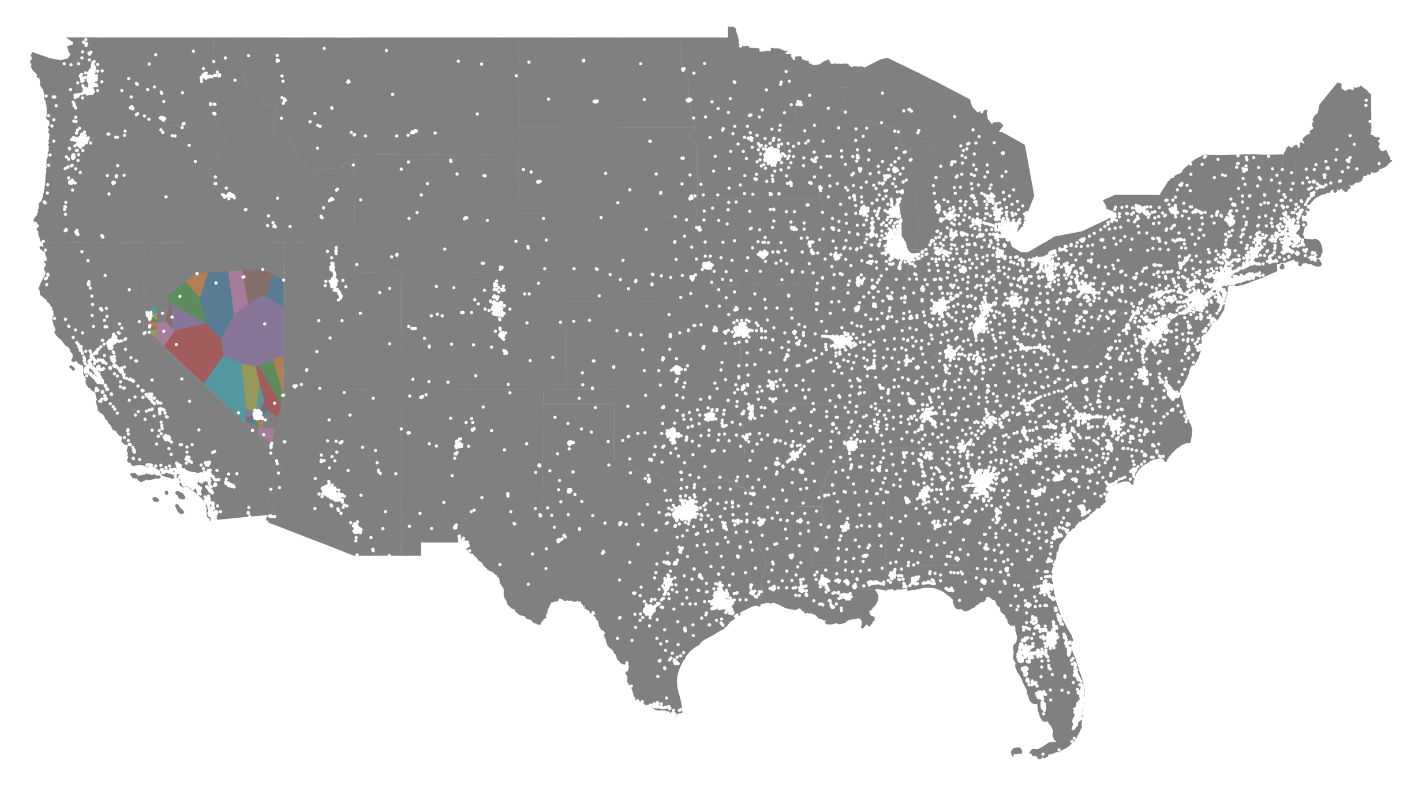
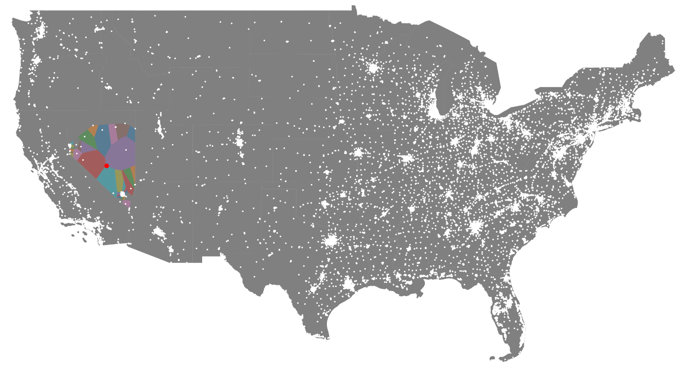
In this example, I'll show what the generated Voronoi diagram looks like for the state of Nevada. I'll show only one state because there are soo many actual locations that the full Voronoi diagram is impossible to make sense of visually.

points = np.array(coords)
vor = Voronoi(points)

regions, vertices = voronoi_finite_polygons_2d(vor)

pts = MultiPoint([Point(i) for i in nv_points])
mask = pts.convex_hull
new_vertices = []

fig, ax = plt.subplots(figsize=(20, 20))

us49.plot(ax=ax, color="grey")

for region in regions:
    polygon = vertices[region]
    shape = list(polygon.shape)
    shape[0] += 1
    p = Polygon(np.append(polygon, polygon[0]).reshape(*shape)).intersection(mask)
    poly = np.array(list(zip(p.boundary.coords.xy[0][:-1], p.boundary.coords.xy[1][:-1])))
    new_vertices.append(poly)
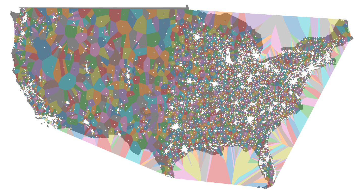
    ax.fill(*zip(*poly), alpha=0.4)
gdf_proj.plot(ax=ax, color="white", markersize=2)

ax.axis('off')

Voilà. Beautiful.

To help make sense of the visual, here's only Nevada and all its restaurant locations, bound by the Voronoi diagram.

So, how do we actually use this information to calculate the McFurthest point?

Time for science!

Now we do the heavy lifting. Our algorithm iterates through all the vertices and ridge vertices in the Voronoi diagram. It checks whether the line segment connecting two vertices intersects the convex hull of the area being considered. If it does, the algorithm calculates the distance from the midpoint of that line segment to the nearest point in the set of US points.

If this distance is less than the current sparsest distance, the midpoint of the line segment is set as the new sparsest point. The algorithm continues iterating through all vertices and ridge vertices, updating the sparsest point and distance as necessary.

import math

def distance(p1, p2):
    return math.sqrt((p1[0] - p2[0])**2 + (p1[1] - p2[1])**2)

convex_hull = us49.unary_union.convex_hull

sparsest_distance = float('inf')
sparsest_point = None

point_regions = [vor.regions[vor.point_region[i]] for i in range(len(vor.points))]

with tqdm(total=len(vor.vertices)) as pbar:
    for i, vertex in enumerate(vor.vertices):
        for j, k in vor.ridge_vertices:
            if j == -1 or k == -1:
                continue
            p1 = vor.vertices[j]
            p2 = vor.vertices[k]
            if convex_hull.contains(Point(p1)) and convex_hull.contains(Point(p2)):
                try:
                    dist = min(distance(p1, points[j]) for j in point_regions[i] if j != -1)
                except IndexError:
                    continue  # ignore the error and continue to the next iteration
                if dist < sparsest_distance:
                    # print(f"New sparsest point: {p1}")
                    sparsest_distance = dist
                    sparsest_point = (p1[0] + p2[0]) / 2, (p1[1] + p2[1]) / 2
        pbar.update(1)

After a grueling 8 hours of crunching numbers (lmao, someone please help me optimize this!) the results are in:

sparsest_point

(-116.36328447653604,38.01828002658917)

Let's see where it is!

fig, ax = plt.subplots(figsize=(20, 20))

us49.plot(ax=ax, color="grey")
ax.plot(sparsest_point[0], sparsest_point[1], 'ro')
gdf_proj.plot(ax=ax, color="white", markersize=2)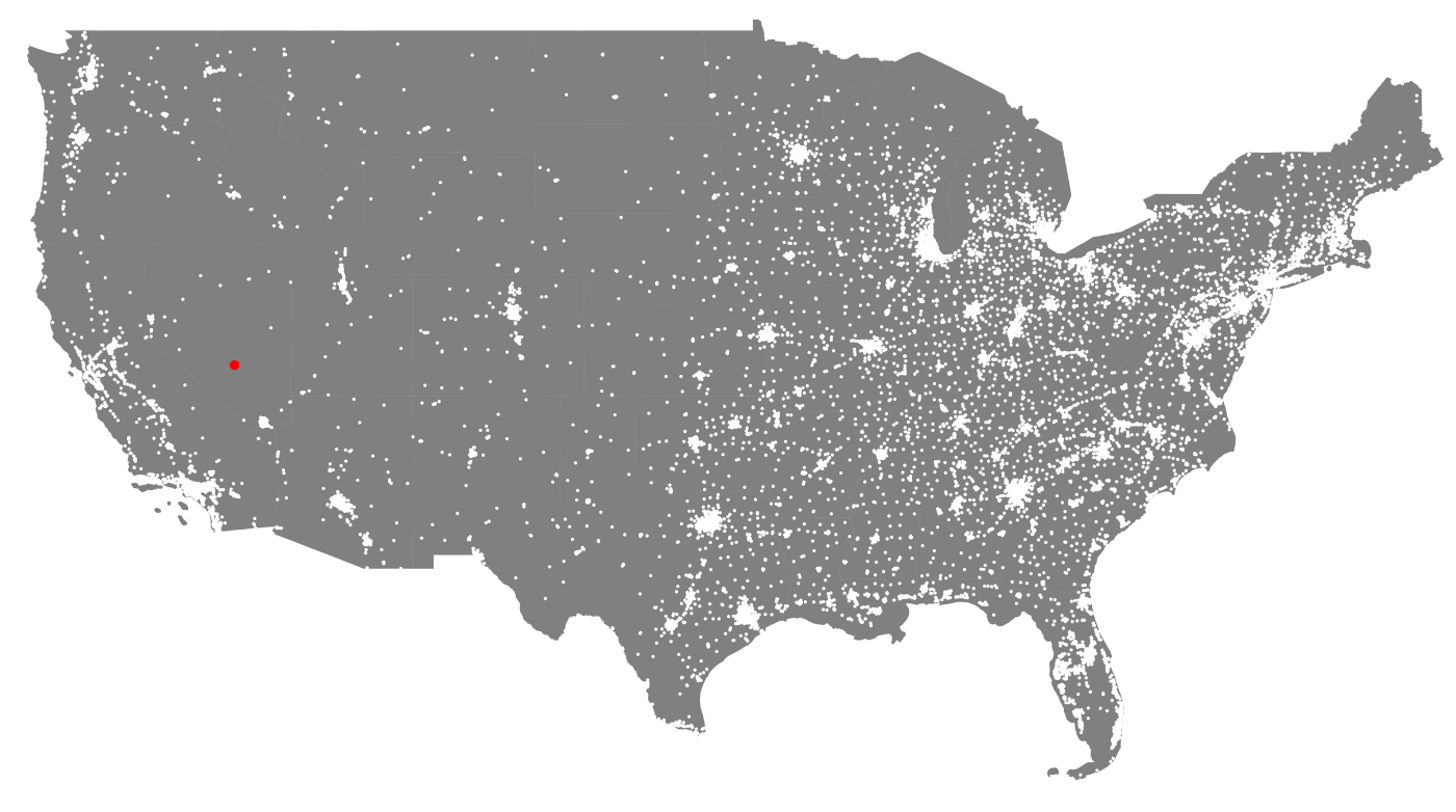

Yep, in the middle of the desert in Nevada!

So, there you have it! Using the power of mathematics and the Voronoi diagram, we can escape the clutches of fast food and find our own little piece of paradise. Now go forth and find your own farthest location from McDonald's!