BigQuery optimization fundamentals

Optimizing SQL queries is essential for businesses to efficiently answer data-related questions and save money. Doing so keeps data consumers happy and ensures that the data is used effectively.

In this article, we will discuss various strategies for optimizing BigQuery queries, including minimizing the data scanned, optimizing aggregation queries, performing efficient joins, and optimizing filtering and ordering.

Primer

First and foremost, the determinants influencing query performance and cost include:

1. The volume of data read by the query in bytes.
2. The amount of data written by your query in bytes.
3. The computational resources, specifically the CPU time, utilized by the query.

One of the most straightforward ways to optimize a query is to limit the number of bytes it needs to scan.

This can be achieved by selecting only the necessary columns and avoiding the use of SELECT *. Since BigQuery uses columnar storage, the data scan is proportional to the number of columns used in the query. If a preview of the data is needed, the preview table feature can be used instead.

Another way to minimize the data scanned in the query is to leverage partitioning and clustering. This involves using filters or where clauses on columns are used to partition or cluster the table itself. By doing so, unnecessary data can be pruned out of the query.

To optimize aggregation queries, it is important to aggregate as late and as seldom as possible. This can be achieved by moving aggregation functions up to the top to avoid multiple group by executions. If a table can be reduced drastically by aggregating in preparation for being joined, it should be aggregated early. Nesting repeated data can also help to avoid using group bys.

When joining multiple tables, it is important to place the largest table first in the join query followed by the smallest and then by decreasing size. Where clauses should be executed as soon as possible to ensure that the slots for forming the join are working with the least amount of data. Filters on both tables should also be used to eliminate unnecessary data. Clustering or partitioning tables based on common join keys can also improve efficiency.

Finally, filtering and ordering can be optimized by choosing the best order for filters in the where clause. The first part of the where clause should always contain the filter that will eliminate the most data. When using an order by statement, it is important to use LIMIT to make the result set easier to manage and avoid overwhelming the processing slot.

By following these optimization strategies, SQL queries can be made more performant and efficient. Now, let's take a deeper look at each of these strategies.

Minimizing Data Scanned

Selecting Specific Columns

One of the most straightforward ways to optimize a query in BigQuery is to limit the number of bytes it needs to scan. This can be achieved by selecting only the columns that are really needed, instead of using "select star".

Since BigQuery uses columnar storage, the data scan is proportional to the number of columns used in the query. Therefore, selecting specific columns can help to minimize the amount of data scanned and improve query performance. If users want to get a feel for the data they are working with, they can use the "preview table" feature to look at the first few rows of the data.

-- Instead of using "SELECT *", specify only the necessary columns
SELECT column1, column2, column3
FROM `project.dataset.table`
WHERE condition;

Using Partitioning and Clustering

Partitioning and clustering are two powerful techniques for optimizing query performance and reducing data scanned in Apache Iceberg tables. These techniques allow you to organize data efficiently, enabling the query engine to quickly identify and process only the relevant data for each query.

Partitioning

Partitioning divides a table into smaller, more manageable segments based on specific column values. This creates a hierarchical structure where data is stored in partitions that correspond to different categories or ranges of values. For instance, a partitioned table storing sales data could be divided into partitions based on the year, month, or date of the sale.

When a query is executed, the query engine can identify the partitions that potentially contain the relevant data. Instead of scanning the entire table, it can focus on the relevant partitions, significantly reducing the amount of data processed. This can significantly improve query execution speed and reduce query costs.

For example, consider a query that retrieves sales data for the month of January 2023. With a partitioned table, the query engine can quickly locate the partitions corresponding to January 2023 and scan only those partitions, avoiding the need to process data from other months.

Clustering

Clustering takes partitioning a step further by physically ordering data within partitions based on another set of columns. This ensures that rows with similar values are stored together on disk. When a query filters or sorts data based on these columns, the query engine can take advantage of this physical order, minimizing data movement and further improving query performance.

For instance, a clustered table for sales data could be sorted by customer ID and product ID. This organization allows the query engine to efficiently retrieve specific customer details or product information, as rows with the same customer ID or product ID will be stored close together.

Example Scenarios

Consider these examples of how partitioning and clustering can be applied to optimize query performance:

• Analyzing sales data by region: Partition the table by date and region to efficiently retrieve sales data for specific regions and time periods.
• Identifying customer demographics: Cluster the table by customer ID and age to quickly retrieve customer information based on age groups.
• Analyzing product performance: Partition the table by product ID and date to efficiently track product sales over time.
• Exploring user behavior: Cluster the table by user ID and activity type to analyze user interactions with specific features or content.

By effectively utilizing partitioning and clustering, you can significantly improve the performance of your queries, reduce data scanned, and lower query costs.

Other strategies

Here are a few other strategies and good practices that you can utilize to minimize data scanned.

• Consider denormalizing data and utilizing nested and repeated fields.
• Create materialized views to efficiently store aggregated data.
• Leverage cached results from previous queries.

Optimizing Aggregation Queries

Understanding Group By Execution

When running aggregation queries in BigQuery, it is crucial to have an understanding of how the system works. First, the data is read from the storage system and grouped into individual slots. Next, a hash function is applied to the results from each slot to group data from the same key together.

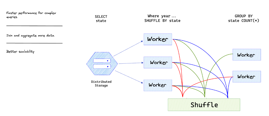
This process is known as shuffling and is visible in the second stage of the execution details. All partial aggregations for the same key end up in the same slot, and further aggregation takes place. Finally, the last slot limits the results and the final result is passed along. Due to the multiple aggregation steps involved, queries can be resource-intensive and costly.

In order to improve the performance of aggregation queries, it is best to aggregate as infrequently and as late as possible. This is particularly relevant for queries that have sub-selects.

To avoid multiple executions and in cases where a table can be significantly reduced by aggregating it before it is joined, it is recommended to move the aggregation functions to the top.

Aggregating Late and Seldom

To avoid using GROUP BY queries, it is possible to nest repeated data. For example, a transactions table that has information about the order, including the items that were purchased, can be denormalized by creating a repeated column that contains a list of all the items. If you want to calculate the number of items in each order, you can use array length and avoid doing any GROUP BY queries.

Assume you have a transactions table with the following structure:

-- transactions table schema
CREATE TABLE my_dataset.transactions (
  order_id INT64,
  order_date DATE,
  items ARRAY<STRUCT<item_id INT64, item_name STRING, quantity INT64>>,
  total_amount FLOAT64
);

Now, let's say you want to calculate the number of items in each order without using a GROUP BY query. You can achieve this by using the ARRAY_LENGTH function:

-- Query to calculate the number of items in each order without GROUP BY
SELECT
  order_id,
  order_date,
  items,
  ARRAY_LENGTH(items) AS number_of_items
FROM
  my_dataset.transactions;

In this example, the ARRAY_LENGTH(items) expression calculates the length of the items array for each row, representing the number of items in the order. This allows you to avoid using GROUP BY for this specific aggregation, as the array functions operate on each row independently.

Note: The denormalization approach with repeated columns should be considered based on the specific requirements and characteristics of your data. It might be beneficial in some scenarios, but it's important to carefully assess the trade-offs, including storage space and query performance.

Smart ordering

Another way to optimize queries is by tweaking the way you do filtering and ordering. When using a WHERE clause, it is important to choose the best order for your filters to eliminate the most data.

If using an ORDER BY statement, it is possible to run into a "resources exceeded" error. This is because the final sorting for your query must be done on a single slot, and if you're attempting to order a very large result set, the final sorting can overwhelm the slot that's processing the data. To solve this, you can use LIMIT so that the result set is easier to manage.

Efficient Joins

Types of Joins in BigQuery

BigQuery supports different types of joins, including hash join or shuffle join, and small join or broadcast join. Hash join or shuffle join is used when two large tables are being joined together. In this case, BigQuery utilizes a hash function to shuffle both the left and right tables so that the matching keys end up on the same worker. This enables the data to be joined locally.

On the other hand, if one of the tables is small enough to fit in memory, it is not necessary to shuffle large amounts of data, and a small join or a broadcast join can be used. In a broadcast join, BigQuery simply sends the small table to every single node that is processing the larger table.

Using Clustering and Partitioning

The already mentioned partitioning and clustering are techniques that can be used to automatically remove unnecessary data from a query, resulting in faster execution. This can be achieved by applying filters or where clauses on columns are used to partition or cluster the table. It is important to minimize the use of GROUP BY queries as they can be very costly. To achieve this, aggregation should be done as late and as seldom as possible.

If a table can be significantly reduced by aggregating it early in preparation for being joined, then that should be done. Another way to avoid using group buys is by nesting repeated data, such as creating a repeated column that contains a list of all the items in a transactions table. By using array length, it is possible to calculate the number of items in each order and avoid doing any group buys.

Join Best practices

Broadcast Joins
When linking a sizable table with a smaller one, BigQuery employs a broadcast join, distributing the smaller table to each processing slot handling the larger table.

Recommendation: Consider using broadcast joins for scenarios where a small table can be efficiently distributed across processing nodes. Place the largest table first, followed by the smallest, and then by decreasing size.

Hash Joins
For merging two extensive tables, BigQuery utilizes hash and shuffle operations to align matching keys in the same slot for local joins. This operation incurs a cost due to the necessary data movement.

Recommendation: Consider clustering to enhance hash join efficiency, particularly when pre-aggregation is part of the query execution plan.

Self Joins
In self joins, a table is merged with itself, often an SQL anti-pattern that can be resource-intensive for large tables, potentially requiring multiple passes.

Recommendation: Favor analytic (window) functions over self joins to reduce query-generated bytes and enhance efficiency.

Cross Joins
Cross joins are deemed an SQL anti-pattern and may lead to considerable performance challenges, generating larger output data than the inputs and, in some instances, causing queries to remain unfinished.

Recommendation: Mitigate performance concerns by using aggregate functions for pre-aggregation or opting for analytic functions, which generally offer superior performance over cross joins.

Skewed Joins
Data skew arises when table partitioning results in unevenly sized partitions. When shuffling data is necessary for joining large tables, skew can cause a drastic imbalance in data transfer between slots.

Recommendation: Pre-filter data at the earliest stage possible or, if feasible, segment the query into two or more queries to address performance issues associated with skewed joins.

Key Takeaways

• Optimizing SQL queries is crucial for businesses to efficiently answer data-related questions and save money.
• Strategies for optimizing BigQuery queries include minimizing data scanned, optimizing aggregation queries, efficient joins, and filtering and ordering optimization.
• By selecting only necessary columns, leveraging partitioning and clustering, and optimizing aggregation queries, businesses can significantly improve their query performance.

Conclusion

Optimizing queries is a complex process that cannot be approached with a one-size-fits-all strategy. It requires a deep understanding of the broader context, including the data structures used, the characteristics of the dataset, and the intricacies of the underlying database system.

Recognizing that optimization is both an art and a science, practitioners need to consider various factors such as data distribution, join strategies, and indexing techniques. The effectiveness of optimization strategies depends on a thorough analysis of the unique context in which the queries operate.