Low-latency trading with Estuary Flow

If you ever decide to venture into the world of real-time data, financial markets provide one of the most interesting, high-volume datasets. Even if you are not interested in trading, it's perfect for building and evaluating stream processing platforms and patterns.

Trading the markets is a wild ride and every split second counts. Imagine you could tap into live market data, implement slick trading strategies, and execute trades with lightning speed – all while seamlessly plugging into your existing data warehousing and notification infrastructure.

That's where Estuary Flow comes in, a real-time data streaming powerhouse.

In this article, we're diving headfirst into building a killer (at least in theory, please don't use this for actual trading!) trading bot with Flow. We'll see how it flexes its real-time ingestion muscles, high-throughput data juggling, and smooth integration capabilities.

Project Overview

To showcase how simple it is to build a real-time operational data pipeline, this project aims to create a simple trading bot capable of ingesting live market data, implementing customizable trading rules, and (almost) executing trades – all while seamlessly integrating with various data and optionally, notification systems.

For good measure, we'll also take a look at how we can save our trades in an analytical warehouse, as we'll need to evaluate the performance of our bot!

All code used in the article is available in this repository.

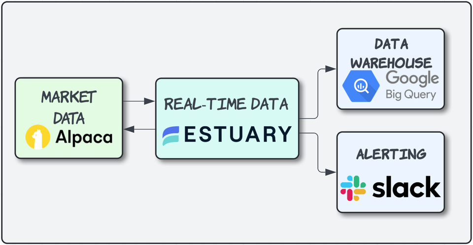
Our whole pipeline consists of four main components:

1. Live market data from Alpaca API

At the market-side of our trading bot lies the integration with Alpaca, a commission-free trading platform renowned for its robust APIs and real-time market data feeds. Through Alpaca's live data stream, our bot will continuously ingest a torrent of up-to-the-second stock quotes, trade executions, and other pertinent market information.

2. Basic trading rules implemented as real-time transformations

While market data provides the raw material, it's the intelligent application of trading rules that imbues our bot with its decision-making prowess. For this project, we'll focus our trading activities on the NVDA stock (NVIDIA Corporation), a prominent player in the tech sector known for its cutting-edge graphics processing units (GPUs) and burgeoning presence in the artificial intelligence realm.

3. Loading events data into BigQuery for further analysis

While the ability to execute trades autonomously is undoubtedly powerful, true trading mastery lies in the ability to analyze and refine one's strategies continuously. To this end, our trading bot will capture and load every triggered buy/sell event, along with relevant trade details, into Google's BigQuery data warehouse.

This centralized event storage and analysis pipeline will empower us to continuously monitor and optimize our trading strategy, identifying potential areas for improvement and making data-driven adjustments to refine our approach over time.

4. Real-time Slack alerts

As an extra, we'll check out how easy it is to set up Slack alerts in our streaming pipeline. Who doesn't love real-time alerting?!

Let's build!

At the core of our pipeline will be Estuary Flow. Flow is a streaming data platform that simplifies the process of building and deploying real-time data pipelines. It provides a user-friendly visual interface for designing data flows, enabling data engineers to construct complex streaming data pipelines with minimal coding efforts.

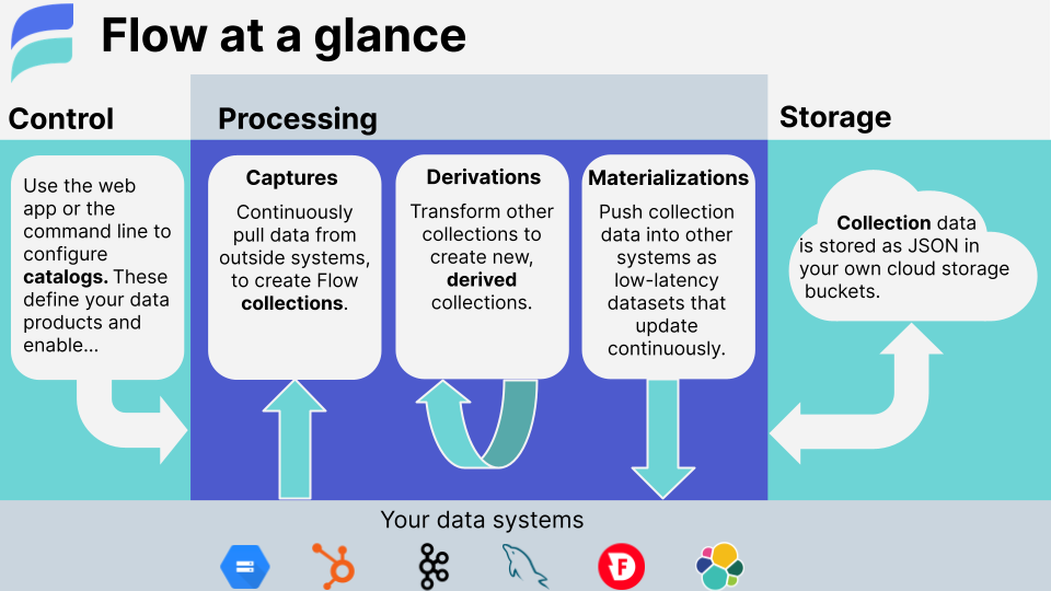
The true power of Flow lies in its vast connector ecosystem, rich transformation capabilities, allowing data to be filtered, enriched, and processed in real-time as it streams through the pipeline.

With its scalability & fault-tolerance Flow empowers teams to build and maintain mission-critical real-time data pipelines with ease, accelerating time-to-value and fostering collaboration through reusable data flow components.

Flow is built on top of the open-source Gazette framework, which does all the heavy-lifting so we don't have to re-invent the wheel!

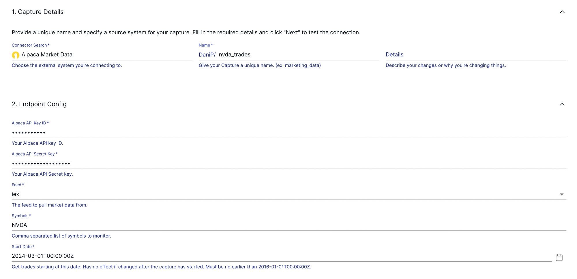
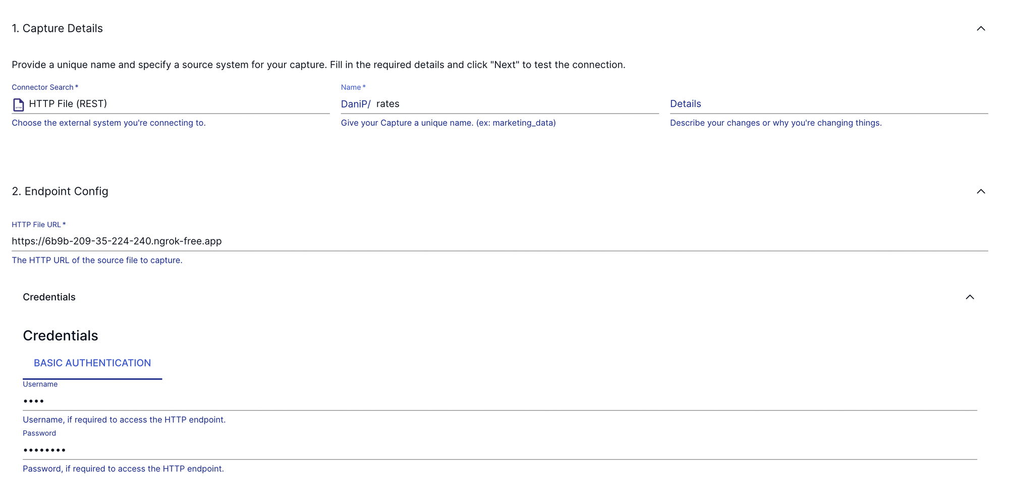
As for our pipeline, first of all, we need data. Lucky for us, Flow comes with a whole lot of ready-to-go, pre-built connectors, such as the one for Alpaca Market Data. After you register an account over at Alpaca and generate an API key, you are ready to provision the data ingestion side of our project.

On the Flow web interface, your configuration will look something like this.

To spice things up a bit, let's integrate some currency exchange data as well to showcase how easy it is to combine integrated datasets downstream in our analytical warehouse.

Create a rates.json file on your machine with the following content:

  {
    "month": "2024-03",
    "USD": 1.0,
    "EUR": 0.88,
    "GBP": 0.75,
    "JPY": 110.45
  }

We'll be using the built-in HTTP file Connector to ingest these values. For Flow to be able to access our local filesystem, we'll need to serve the directory containing the exchange rate values. This can be very easily done via a tool, like ngrok:

ngrok http --basic-auth="user:password" file:///path/to/rates

Ngrok will spin up a fileserver locally and give you a URL that you can paste into the configuration window on the Estuary UI.

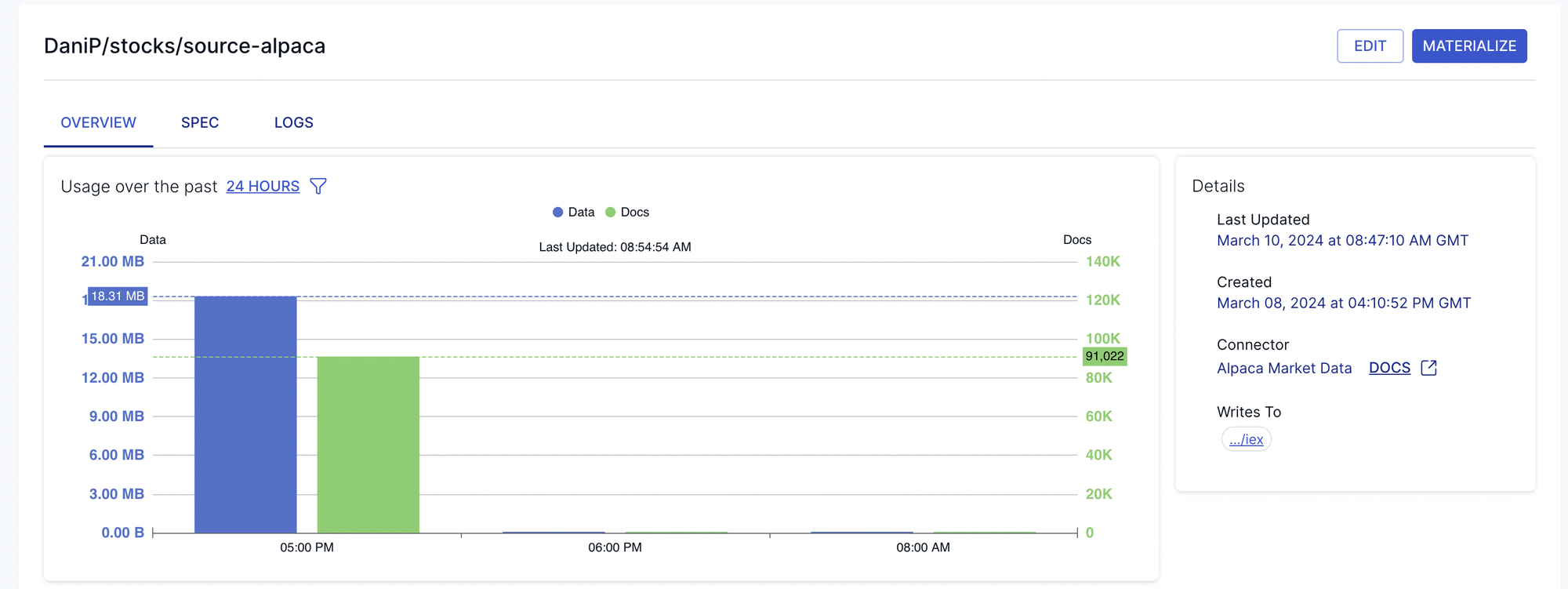
That's it! Now we have two sources configured and data is rolling in. To verify, check out the details page of each source. You should see something like this:

Transformations

Alright, data is is flowing. The next step is to codify our trading strategy. We can do this by implementing derivations.

Estuary Flow's derivations are powerful constructs that enable continuous, low-latency transformations on real-time data streams. They allow you to perform a wide range of operations, from simple remappings to complex, stateful data processing. As new data flows in, derivations automatically recalculate and propagate the transformed results, ensuring downstream applications always have access to the latest, accurately processed information.

This real-time data transformation capability opens up possibilities for building sophisticated event-driven architectures, complex enrichment pipelines, and stateful systems reacting to evolving data.

Writing transformations is hard. Writing real-time transformations is even harder! Thankfully, Flow provides two simple, familiar interfaces for us: SQL and Typescript. For this project, we'll look at what SQL transformations look like.

The first step is to set up your local development environment.

1. Authenticate flowctl

flowctl auth login

2. Pull existing resource definitions from the Flow web service. (These include the sources we created on the UI in the previous steps!)

flowctl catalog pull-specs

At this point, your working directory should look something like this

~/estuary-project main ❯ tree
.
├── DaniP
│   ├── flow.yaml
│   ├── rates
│   │   ├── flow.yaml
│   │   ├── rates.schema.yaml
│   │   └── source-http-file.config.yaml
│   └── stocks
│       ├── flow.yaml
│       ├── iex.schema.yaml
│       └── source-alpaca.config.yaml
├── flow.yaml
└── rates
    └── rates.json

A few notes on the resource hierarchy of Flow before we continue.

• Catalog: The set of published entities that comprise all Data Flows, including captures, materializations, derivations, collections, schemas, tests, etc.
  • Data Flows: Combinations of catalog entities to create various Data Flows.
    • Capture: Captures data from sources.
• Collection: Organizes captured data.
• Derivation: Transforms organized data into new collections.
• Materialization: Produces derived data into a specified destination.
• Flow specification files: YAML files containing configuration details for catalog entities, created either through the web app or using flowctl.
  • Namespace: All catalog entities identified by a globally unique name with directory-like prefixes.
    • Prefixes: High-level organizational prefixes are provisioned for the organization, akin to database schemas for table organization and authorization.
      • Example: acmeCo/teams/manufacturing/
      • Example: acmeCo/teams/marketing/

Alright, with that out of the way, let's continue. After pulling the existing capture and collection definitions from Flow, this is how our flow.yaml should look like:

---
captures:
  DaniP/stocks/source-alpaca:
    autoDiscover:
      addNewBindings: true
      evolveIncompatibleCollections: true
    endpoint:
      connector:
        image: "ghcr.io/estuary/source-alpaca:v1"
        config: source-alpaca.config.yaml
    bindings:
      - resource:
          name: iex
        target: DaniP/stocks/iex
    shards:
      disable: true

collections:
  DaniP/stocks/iex:
    schema: iex.schema.yaml
    key:
      - /ID
      - /Symbol
      - /Exchange
      - /Timestamp

As you can see, we have a capture and a collection definition, nothing fancy (so far). Now, we can create a new collection, which will have one derivation attached to it.

To do this, simply extend the yaml file with the following stanza

collections:
  DaniP/stocks/iex:
    schema: iex.schema.yaml
    key:
      - /ID
      - /Symbol
      - /Exchange
      - /Timestamp

  DaniP/stocks/dips:
    schema: dips.schema.yaml
    key:
      - /ID
      - /Symbol
      - /Timestamp

    derive:

      using:
        sqlite: {}

      transforms:
        - name: checkThreshold
          source: DaniP/stocks/iex
          shuffle: { key: [/Symbol] }
          lambda: checkThreshold.sql

Our derived collection is aptly named DaniP/stocks/dips as its purpose is going to be to look for dips in the market data, according to our strategy. Create the checkThreshold.sql file next to the flow.yaml you are editing and add the following to it:

SELECT $ID, $Symbol, $Exchange, $Timestamp, $Price WHERE $Price < 835;

This transformation defines our trading "strategy". Feel free to go crazier in your implementation!

Based on the SQL query above, we can create a schema definition file for the new collection, called dips.schema.yaml.

Before publishing our transformation, let's test it locally with flowctl.

~/estuary-project main* ❯ flowctl preview --source flow.yaml --name DaniP/stocks/dips                                                            

{"ID":3299,"Price":834.29,"Symbol":"NVDA","Timestamp":"2024-03-05T15:42:24.637731686Z"}
{"ID":3300,"Price":834.47,"Symbol":"NVDA","Timestamp":"2024-03-05T15:42:24.657427966Z"}
{"ID":3301,"Price":834.52,"Symbol":"NVDA","Timestamp":"2024-03-05T15:42:24.658964833Z"}
{"ID":3302,"Price":834.52,"Symbol":"NVDA","Timestamp":"2024-03-05T15:42:24.65898575Z"}
{"ID":3303,"Price":834.53,"Symbol":"NVDA","Timestamp":"2024-03-05T15:42:24.65899521Z"}
{"ID":3304,"Price":834.51,"Symbol":"NVDA","Timestamp":"2024-03-05T15:42:24.660216814Z"}
{"ID":3305,"Price":834.53,"Symbol":"NVDA","Timestamp":"2024-03-05T15:42:24.660245915Z"}

Nice, looks like there are a bunch of opportunities for buying the stock according to our rule! Let's publish the derivation with flowctl catalog publish --source flow.yaml.

To trigger the actual buy event at our broker, we have two ways to go forward.

1. We can use the HTTP webhook destination to send the buy orders to an API.
2. We can call the API directly from a transformation through a custom Typescript function, using the broker's client library.

The live trading part is slightly out of scope for this article, but check back later, when we'll showcase how to work with Typescript functions!

Destinations

It's usually preferable to consolidate your data sources in a data warehouse for further analysis. Warehouses, such as BigQuery offer the cheap storage and scalable compute required for large-scale analytics on historical data, which would get really tricky in a streaming environment.

For this purpose, we'll load our two datasets into BigQuery. To set this up, we can head back to the Flow UI and configure the BigQuery materialization.

To join our two collections (dips and exchange rates), let's add both to the materialization configuration.

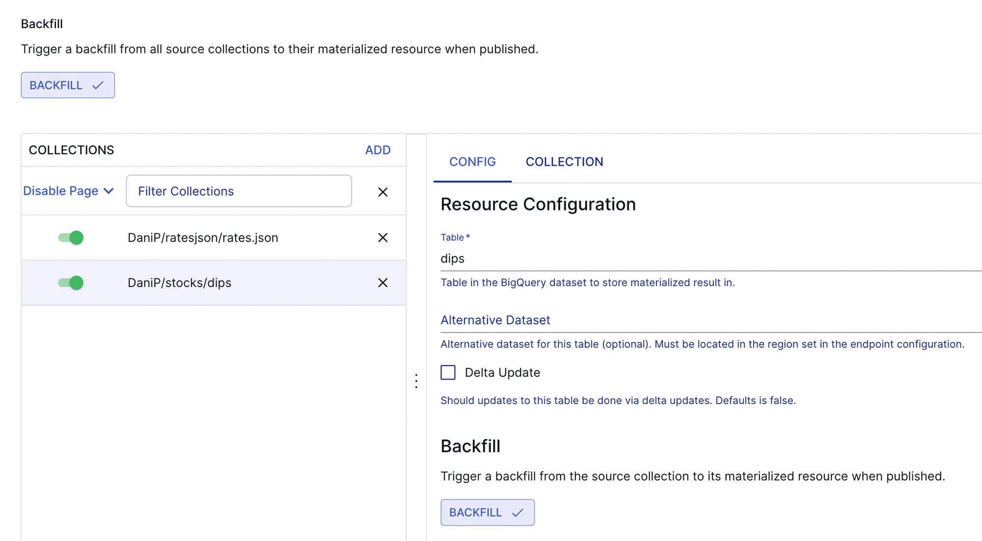
To make sure you version control every component of your pipeline, don't forget to pull the latest specifications locally! Your working directory at the end should look something like this:

~/estuary-project main* ❯ tree                                                                                                                 
.
├── DaniP
│   ├── dwh
│   │   ├── flow.yaml
│   │   └── materialize-bigquery.config.yaml
│   ├── flow.yaml
│   ├── ratesjson
│   │   ├── flow.yaml
│   │   ├── ratesjson.schema.yaml
│   │   └── source-http-file.config.yaml
│   └── stocks
│       ├── checkThreshold.sql
│       ├── flow.yaml
│       ├── iex.schema.yaml
|       ├── dips.schema.yaml
│       └── source-alpaca.config.yaml
├── flow.yaml
└── rates
    └── rates.json

After configuring access with a service account, let's head over to the BigQuery console to analyze our orders! At the moment of writing this, let's say NVDA trades at €860 (or ~$940).

with buys as (
  select
  Symbol,
  Timestamp,
  Price AS price_usd,
  round(Price * rates.EUR) AS price_eur
FROM
  `sandbox.estuary.iex` trades
  join `sandbox.estuary.rates_json` rates on EXTRACT(MONTH FROM trades.Timestamp) = EXTRACT(MONTH FROM PARSE_DATE("%Y-%m", rates.month))
)

, buys_per_symbol as (
  select
    Symbol,
    count(*) as num_buys,
    sum(price_usd) as total_usd,
    sum(price_eur) as total_eur
  from buys
  group by Symbol
)

, profit as (
  select
    Symbol as symbol,
    (num_buys * 940) - total_usd as profit_usd
    (num_buys * 860) - total_eur as profit_eur
  from buys_per_symbol
)

select * from profit;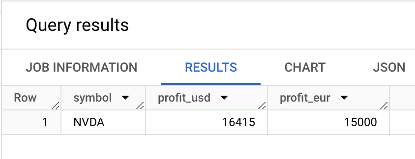

Aaaand it looks like our trading bot would have made us around €15000 if it had been running since the first of March! Not bad, but obviously, it helped that the stock was skyrocketing during this time.

To demonstrate how useful it can be to fan out to destinations for the same processing pipeline, we can also look at setting up Slack alerts using the same collections.

This is as simple as configuring a Slack destination that will trigger messages on new records in our orders collection, meaning we'd get a notification every time our bot executes a buy order!

Conclusion

Estuary Flow emerges as a powerful solution for data engineers tasked with building robust and efficient real-time data pipelines for not just algorithmic trading systems, but anything requiring integrating multiple data sources, transforming them dynamically, and preparing them for operational analytics or AI.

Throughout this project, we have witnessed Estuary's prowess in seamlessly handling low-latency data ingestion from sources like Alpaca API, enabling the capture of up-to-the-second market data streams. Coupled with its high-throughput data processing capabilities, Flow empowers data engineers to implement complex trading rules and logic, ensuring that data reliably arrives at the destination.

Moreover, Estuary's rich integration features streamline the process of connecting disparate systems, such as loading trade event data into BigQuery for comprehensive analysis or setting up Slack alerts. These seamless integrations eliminate the need for complex custom code, allowing data engineers to focus on delivering value rather than wrestling with intricate system interconnections.

By abstracting away the complexities of real-time data ingestion, transformation, and integration, Estuary Flow empowers data engineers to concentrate on building sophisticated trading strategies and delivering robust, scalable systems that can adapt to evolving market dynamics.